Welcome, readers! In the last Wireshark 101 article, we installed Wireshark and got introduced to the interface. This time we are diving in and analyzing our first packets! I’m using Windows 7 in this tutorial, so following along will be easiest if you are using Windows yourself. Also noteworthy is the fact that I’m using a computer plugged into an Ethernet II network. If you are using wireless or a different layer 2 wired technology other than Ethernet II (unlikely, but possible), you’ll have a different experience than what is depicted, but feel free to follow along anyway! Go ahead and fire up Wireshark and start a new live capture by choosing your capture interface and clicking the green shark icon. Once the capture’s going, open up cmd.exe by pressing Windows Key+R, typing “cmd.exe” without the quotes, and pressing enter. Now type the following command to send 4 ICMP (Internet Control Message Protocol) packets to 8.8.8.8, Google’s public DNS server:
ping 8.8.8.8
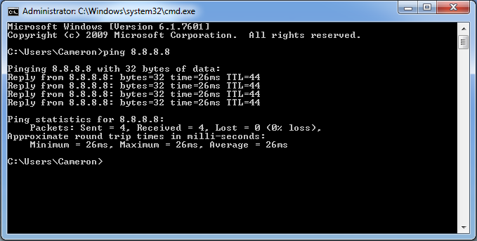
This command will send 4 ICMP Echo Request (“ping”) packets to the IP address 8.8.8.8. Your screen should look pretty much like the window below.
After the pings have been sent, minimize cmd.exe, pull Wireshark back up and stop the capture by pressing the red stop button just beside the green shark fin. Now let’s go back to the cmd.exe window so we can discuss our results. A ping is a low level network packet that, among other things, is often used to test basic connectivity to a network device. Each echo request ping packet is a humble request that the receiving device respond back. The fact that you received a response to your pings is a confirmation that we have a path from your computer to 8.8.8.8, a path from 8.8.8.8 back to your computer, and that the device that responded is being nice and not ignoring or blocking our pings. The ping does not tell us who 8.8.8.8 is or where it is located or what services it offers. We just happen to know in advance that this is Google’s Public DNS server (with that in mind, please don’t spam the server by sending more pings than are necessary for the purposes of this tutorial).
In the cmd.exe window, we are given some information about the response back from our pings. The first line after our command tells us which IP address we are pinging and how many “bytes of data” are being sent in each packet. The next four lines detail the responses we received from each ping packet. The address where the reply originated, the amount of data bytes that were received, the amount of time it took for the response to return in milliseconds, and the TTL (Time to Live) value for each packet are seen in each line, from left to right. At the bottom of our window, we see some summary statistics.
Let’s switch back over to the Wireshark window. If any applications on your computer were sending network traffic while you performed your packet capture, or if there were noisy broadcasting devices on your network, you’ve likely got extra packets besides the 8 we are looking for in your trace file. The filter field is going to help us solve this “needle in the haystack” issue. Simply type “icmp” without quotes into the filter field and press enter. As long as there were no other ICMP packets sent during your capture, you should now have a window very similar to this:
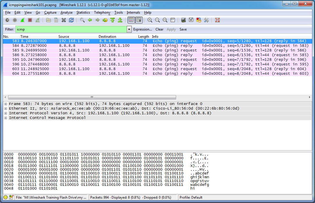
Wow, this is much easier to deal with! Notice that the filter field turns green since we have typed an appropriate display filter pattern. Alright, so what are we looking at here? Each row in the packet list pane corresponds to a single packet. Currently, and for reasons we’ll explore later on, each packet is colored pink (the top packet is blue since it is selected). Follow along by referencing the first packet in the list (No. 583, the blue one). The columns in the packet list pane denote the following pieces of information:
No.: The number of the packet within the capture file. Wireshark counts packets in the order that they were received, starting with number 1. Packet 583 would be the 583rd packet that Wireshark saw since beginning its capture. The packet numbers in this picture aren’t sequential because we have applied a display filter to only show ICMP traffic. It just so happens that other packets were received between the pings, and the pings began after 582 packets were already captured.
Time: The time that the packet was received in seconds after the capture was started. A time value of 8.246 indicates that Wireshark received this packet 8.246 seconds after the capture began.
Source: The source IP address of the packet. This first packet originated from 192.168.1.100, which happens to be the internal IP address of my home computer. Wireshark captured this packet as it left the computer.
Destination: The destination IP address of the packet. This first packet was addressed to be delivered to 8.8.8.8.
Length: The length of the packet in bytes. Each of these packets is 74 bytes in length.
Info: Some relevant information about the packet depending on what protocol is being used. In this instance, Wireshark has determined that these are ICMP ping packets, and has displayed whether each packet is an ICMP echo request or reply, the id and sequence values of each packet, the TTL value for each packet, and the packet number of the accompanying reply (if it’s a request) or the packet number of the accompanying response is (if it’s a reply).
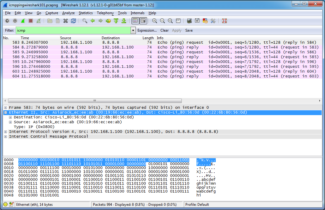
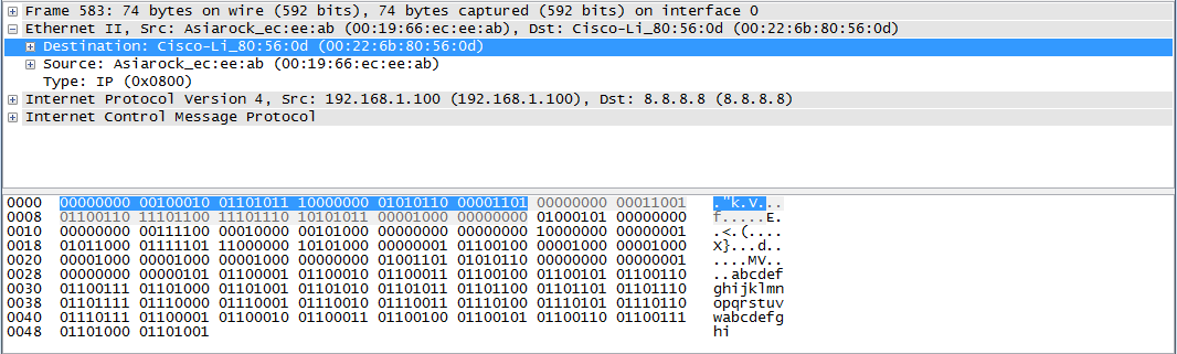
Let’s dive further into this first packet. With the first packet highlighted in the packet list pane, we’ll move our attention to the packet details pane in the middle of the screen. Each row corresponds to a layer of the packet and essentially, a particular protocol. The first layer (Frame xxx…) corresponds to the physical layer of the OSI model. The only important thing we need to know about the layer 1 information is that Wireshark received a string of bytes called a preamble indicating that an Ethernet II frame header was coming up. Feel free to investigate this layer, but we won’t be discussing it–we’re going straight to layer 2! Click on the the little plus sign to the left of “Ethernet II…” to expand the Ethernet II header. What we see is a destination and source address, and a “Type” field. These destination and source addresses are known as Media Access Control (MAC) addresses, and they are used to identify devices at layer 2 of the OSI model. Each MAC address is 6 bytes or 48 bits in length and corresponds to a particular hardware interface. The first 3 bytes (the first half) of the MAC address is known as the Organizational Unique Identifier (OUI) and identifies the name of the organization which manufactured the network interface card (NIC). There’s an option in Wireshark to check OUI’s against a database and display the name of the company that manufactured the NIC–that’s why in my capture file we can see “Asiarock” and “Cisco-Li” (Cisco-Linksys). The non-interpreted MAC address is shown in full in parenthesis to the right of the interpreted addresses. The Type field designates what type of protocol will be coming up after the Ethernet II header. In my case, it is IP (Internet Protocol version 4), which you can confirm by looking at the layer directly beneath the Ethernet II header.
If you select a line from the packet details pane, the corresponding bytes will also be highlighted in the the packet bytes pane. I’ve just realized that the default setting for the packet bytes pane is to display the bytes in hexadecimal, and I’m viewing mine in binary. To switch between the two views, right click anywhere in the packet bytes pane and choose “Bits View”. In the picture above, I have selected the entire Ethernet II header by clicking the text on the line rather than the plus symbol (see the blue line in the packet details pane in the picture above). By doing this, we can see every byte and bit that comprises the Ethernet II header and it’s ASCII interpretation (which isn’t that interesting for this part) in the packet bytes pane highlighted in blue. As expected, the Ethernet II header is 14 bytes in length (14 sets of 8 bits, or one hundred and twelve 1’s and 0’s–go ahead, count them yourself!). It all adds up considering we know that there is a destination MAC address (6 bytes), a source MAC address (6 bytes) and a Type field (2 bytes). You could also select any of these fields to see their corresponding bytes in the packet bytes pane. In the picture below, I’ve selected the Destination MAC address and the corresponding 6 bytes are highlighted:
If you understand how to convert binary to hexadecimal, you’ll see that the binary and hexadecimal do indeed match up. And even if you don’t know how to convert binary to hexadecimal, you can switch to hexadecimal view in the packet bytes pane. Keep in mind that the bits we see in the packet bytes pane are the result of the actual electrical signals sent across the wire which correspond to 1’s and 0’s. Wireshark applies dissectors to these bit streams in order to know which bits and bytes correspond to particular pieces of information. For instance, when we evaluate the first six bytes of the Ethernet II header, we see that we can convert it to hexadecimal as 00:22:6b:80:56:0d. There is nothing in these bytes that translates into the text “Destination” or “Cisco-Li_”. Wireshark knows that this is a destination MAC address because it has applied a dissector which specifies that the first 6 bytes of the Ethernet II header are to be interpreted as a destination MAC address. This same group of bytes would be interpreted differently if it were located in a different place in the packet. Likewise, “Cisco-Li_” is the OUI which is supplied by Wireshark after checking an OUI dictionary. There is no information located within the bytes themselves that would provide this knowledge. Additionally, Wireshark knew to apply it’s Ethernet II dissector to this section of the packet due to the preamble it received indicating that an Ethernet II header was coming up. This is one of the beautiful things about Wireshark. You are able to quickly access a ton of information without having to know the protocols inside and out and without having to manually compute what each bit and byte means.
Whew! This is shaping up to be a two-parter. Go ahead and save your Wireshark capture by choosing File > Save As… and choosing a place to save the file. Next week we’ll use this same file to examine the rest of the packet. Thanks for reading!